Figure showing the robustness for stickleback

Name of this file: Cuaderno20120402T211533.m

fig_pap_robustezstickleback(1,[0 0 0])

 

Repetition of stickleback figures, with new fits

Name of this file: Cuaderno20120402T124252.m

Now that we know that the model has an analytical relation with the one in the PLoS, it makes sense to use for the case k=1 the parameters that correspond to those in the PLoS. So I repeat the figures with the new parameters.

Load data

load datos_wardetal

Symmetric case, re-fit of a for k=0.5

I fix k=0.5 and s=2.5. I refit a.

params_stickleback.a=3;
params_stickleback.s=2.5;
params_stickleback.k=.5;
params_stickleback.sigma=params_stickleback.s^-params_stickleback.k;
params_stickleback.sigmaundecided=0;
params_stickleback.p_rand=0;
a=10.^(-5:.05:5);
n_a=length(a);
logprob=NaN(1,n_a);
for c_a=1:n_a
params_stickleback.a=a(c_a);
[logprob(c_a),rootmeansqerr,handles,hist_modelo,logprob_cadahist]=comparadatos_papersara(datos_wardetal.sinpredador,params_stickleback,0);
end % c_a
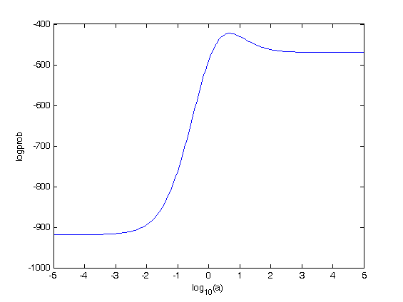
plot(log10(a),logprob)
xlabel(‘log_{10}(a)’)
ylabel(‘logprob’)
[m,ind]=max(logprob);
a_opt=a(ind)

a_opt =
5.0119

 

Symmetric case, re-fit of a for k=0

I fix k=0 and s=2.5. I refit a.

params_stickleback.s=2.5;
params_stickleback.k=0;
params_stickleback.sigma=params_stickleback.s^-params_stickleback.k;
params_stickleback.sigmaundecided=0;
params_stickleback.p_rand=0;
a=10.^(-5:.05:5);
n_a=length(a);
logprob=NaN(1,n_a);
for c_a=1:n_a
params_stickleback.a=a(c_a);
[logprob(c_a),rootmeansqerr,handles,hist_modelo,logprob_cadahist]=comparadatos_papersara(datos_wardetal.sinpredador,params_stickleback,0);
end % c_a
plot(log10(a),logprob)
xlabel(‘log_{10}(a)’)
ylabel(‘logprob’)
[m,ind]=max(logprob);
a_opt=a(ind)

a_opt =
223.8721

 

With predator, re-fit of ax, ay for k=0.5

params_stickleback.s=2.5;
params_stickleback.k=.5;
params_stickleback.sigma=params_stickleback.s^-params_stickleback.k;
params_stickleback.sigmaundecided=0;
params_stickleback.p_rand=0;
a=10.^(-5:.1:5);
n_a=length(a);
logprob=NaN(n_a);
for c_ax=1:n_a
for c_ay=1:n_a
params_stickleback.a=[a(c_ax) a(c_ay)];
[logprob(c_ay,c_ax),rootmeansqerr,handles,hist_modelo,logprob_cadahist]=comparadatos_papersara(datos_wardetal.conpredador,params_stickleback,0);
end % c_ay
end % c_ax
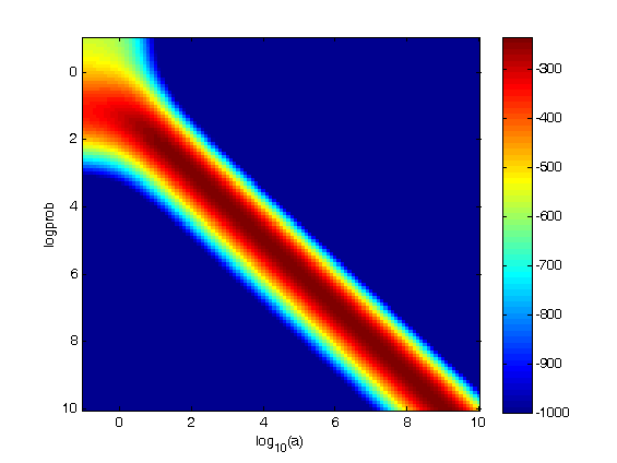
imagesc(log10(a),log10(a),logprob)
xlabel(‘log_{10}(a)’)
ylabel(‘logprob’)
colorbar
[m,ind]=max(logprob(:));
[i,j]=ind2sub(size(logprob),ind);
ax_opt=a(j)
ay_opt=a(i)

ax_opt =
1.2589
ay_opt =
31.6228

 

With predator, re-fit of ax, ay for k=0

params_stickleback.s=2.5;
params_stickleback.k=0;
params_stickleback.sigma=params_stickleback.s^-params_stickleback.k;
params_stickleback.sigmaundecided=0;
params_stickleback.p_rand=0;
a=10.^(-1:.1:10);
n_a=length(a);
logprob=NaN(n_a);
for c_ax=1:n_a
for c_ay=1:n_a
params_stickleback.a=[a(c_ax) a(c_ay)];
[logprob(c_ay,c_ax),rootmeansqerr,handles,hist_modelo,logprob_cadahist]=comparadatos_papersara(datos_wardetal.conpredador,params_stickleback,0);
end % c_ay
end % c_ax
imagesc(log10(a),log10(a),logprob)
xlabel(‘log_{10}(a)’)
ylabel(‘logprob’)
caxis([-1000 m])
colorbar
[m,ind]=max(logprob(:));
[i,j]=ind2sub(size(logprob),ind);
ax_opt=a(j)
ay_opt=a(i)

ax_opt =
1.2589e+009
ay_opt =
1.0000e+010

 

Figure in the main text

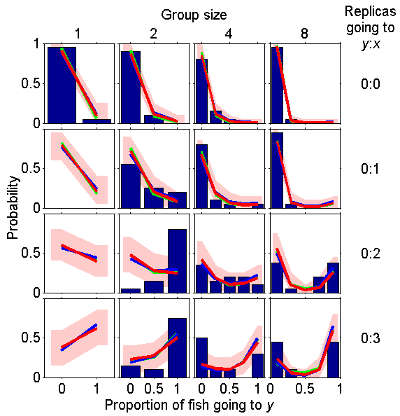
fig_pap_stickleback(1)

 

Oops! It turns out that with the new parameters the non-predator fit is not very good. Indeed, in the PLoS this is one of the worst cases. The fit was better with the old parameters.

Supplementary figures

fig_pap_sticklebacksuppl(2,1)
fig_pap_sticklebacksuppl(3,2)
fig_pap_sticklebacksuppl(4,3)

 

 

 

Relation between the new model (the one in Sara’s paper) and the old one (the one in PLoS). It is analytical!

Name of this file: Cuaderno20120402T111150.m

Model definition

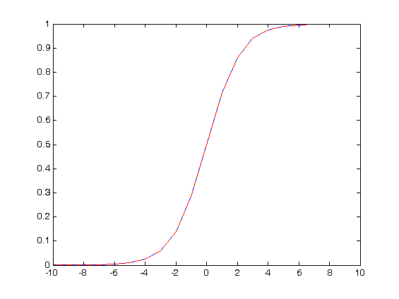
I define the new model with k=1, so that we have deltan

P=@(ax,ay,s,deltan) (1+(1+ax*s.^-deltan)./(1+ay*s.^deltan)).^-1;
Pold=@(a,s,deltan) (1+a*s.^-deltan).^-1;

Comparison for a=1

They are identical

figure
deltan=-10:10;
a=1;
s=2.5;
ax=1;
ay=1;
plot(deltan,Pold(a,s,deltan))
hold on
plot(deltan,P(ax,ay,s,deltan),’r–‘)

 

Comparison for a~=1

I check for a=10.

figure
deltan=-10:10;
a=10;
s=2.5;
ax=1;
ay=.1;
plot(deltan,Pold(a,s,deltan))
hold on
plot(deltan,P(ax,ay,s,deltan),’r–‘)

aes=10.^(-5:.1:5);
n_a=length(aes);
errores1=NaN(n_a);
for cx_a=1:n_a
for cy_a=1:n_a
errores1(cy_a,cx_a)=sum(abs(Pold(a,s,deltan)-P(aes(cx_a),aes(cy_a),s,deltan)));
end % cy
end % cx
[m,ind]=min(errores1(:));
[i,j]=ind2sub(size(errores1),ind);
ax=aes(j)
ay=aes(i)
figure
imagesc(log10(aes),log10(aes),errores1)
colorbar
figure
imagesc(log10(aes),log10(aes),log10(errores1))
colorbar
xlabel(‘log_{10}(a_x)’)
ylabel(‘log_{10}(a_y)’)
figure
plot(deltan,Pold(a,s,deltan))
hold on
plot(deltan,P(ax,ay,s,deltan),’r–‘)

ax =
10
ay =
0.1000

 

 

 

 

So we get a very clear minimum, with excellent agreement.

General search for a~=1

I repeat the whole procedure for different values of a.

a=10.^(-5:.5:5);
m=NaN(length(a),1);
ax=m;
ay=m;
for c_a=1:length(a)
aes=10.^(-5:.1:5);
n_a=length(aes);
errores2=NaN(n_a);
for cx_a=1:n_a
for cy_a=1:n_a
errores2(cy_a,cx_a)=sum(abs(Pold(a(c_a),s,deltan)-P(aes(cx_a),aes(cy_a),s,deltan)));
end % cy
end % cx
[m(c_a),ind]=min(errores2(:));
[i,j]=ind2sub(size(errores2),ind);
ax(c_a)=aes(j);
ay(c_a)=aes(i);
end % c_a
subplot(1,2,1)
plot(log10(a),log10(m))
xlabel(‘log_{10}(a_{old})’)
ylabel(‘log_{10}(error)’)
subplot(1,2,2)
hold off
plot(log10(a),log10(ax))
hold on
plot(log10(a),log10(ay),’r’)
xlabel(‘log_{10}(a_{old})’)
ylabel(‘log_{10}(a_{new})’)

 

figure
loglog(a,ax./ay,’.-‘)
xlabel(‘a_{old}’)
ylabel(‘a_x/a_y’)
figure
loglog(a,ax)
xlabel(‘a_{old}’)
ylabel(‘a_x’)
figure
loglog(a,ay)
xlabel(‘a_{old}’)
ylabel(‘a_y’)
figure
loglog(ax,ay)
xlabel(‘a_x’)
ylabel(‘a_y’)

 

 

 

 

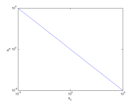
So incredibly simple relation! There must be something analytical here…

Efectiviguonder

It turns out that

.

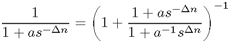So it is analytical! We just have ax=a, ay=1/a.